The Gaming of LEED Ratings

We all know that the LEED system can be gamed but that it could be turned so completely on its head was news to me.

greenwashThe Bank of America building at One, Bryant Park, New York has a LEED Platinum rating and was the first skyscraper to ever be awarded this but now, it turns out, it uses more energy per square foot than other building of similar size in all of Manhattan. Wow.

It was hailed as a major achievement by none other than Al Gore who set up his offices there. The basic problem is that LEED is largely based on computerised energy models and “intent”. This makes it open to abuse because it’s easy to purportedly intend something at the design stage and then change the goalposts later on.

Coincidentally, just this morning, I was speaking to a couple of marketing guys who were trying to convince me to attend a “green summit” next month and one of their selling points was LEED. I declined, telling them exactly what I thought of LEED but I wish I’d seen this article just a few hours earlier:

Bank of America Tower and the LEED Ratings Racket via: ArchRecord
Conditional Formatting

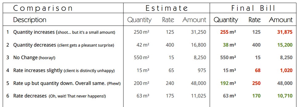
Yesterday, a contractor submitted his bill for some work that had been carried out and, not surprisingly, it was a little different from the original estimate. I often make an extra set of columns in the spreadsheet to show the bill and estimate alongside each other. This way the client can easily see what has changed.

On this occasion, I decided to do a little more; I decided to colour-code the changes in the bill vis-a-vis the estimate. It could be done manually, of course but this can quickly become tedious if you have anything more than a handful of cells to format.  Instead, we can let the spreadsheet do the grunt work.  After all, that’s what it’s there for.

Here is a brief outline of how it is done so anybody (my future self included) can see how to do it.  The instructions are for LibreOffice but they couldn’t be that different for Excel.

Here are the steps in brief.

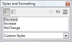
Three Styles

Set up the styles using the style manager (F11). I created three with different colours.

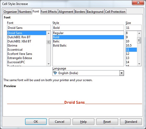
Style Formatting

Modify the font, colour and background to suit your requirements

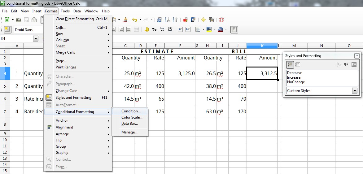
Menu

Click the cell where you want to format to be applied (K3 in this example) then go to Format>Conditional Formatting>Condition…

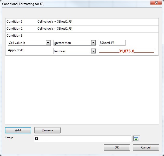
Conditions for K3

And add the three conditions

TIP: If the cell for comparison is listed as $F$3 that means it is an absolute value. If, however, you remove the $ signs, it will refer to a cell placed relative to the one where the condition is applied.

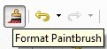
Format Paintbrush

Format Paintbrush

Once you have a cell set up the way you want, simply use the format paintbrush to apply it to other cells.

The Output

And finally, here is a sample of the output